Computational photography: M-Kamera and GrainWorks

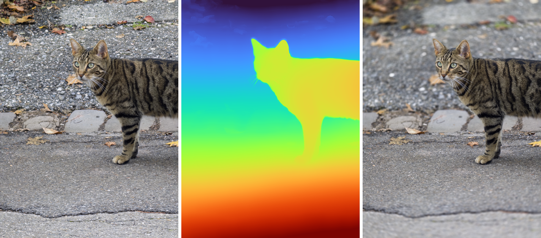
If you read my post about M-Kamera, you know that for me photography is as much about the process as about the results: preferably slow, mechanical, and with a fair chance of things going wrong both in the field and in the darkroom. In other words, analogue photography 🙂

M-Kamera is my attempt to simulate this process on a phone as closely as possible, down to the actual physics of grain and lens (just try the hardcore mode!). I think it works to some degree, though a real film advance and a physical focus ring are obviously still a work in progress, and always will be. In any case, there’s nothing like it, so give it a try!

On the other hand, M-Kamera is niche by design: even some 35mmc readers find it too extreme. That’s why it also has a simplified P&S mode for non-geeks (my 18-year-old daughter uses it as her main camera app). One fundamental, and deliberate, limitation will always be there: M-Kamera only works on pictures taken with M-Kamera, with all the (simulated) limitations of analogue photography attached. Not everyone cares about the process, so for those of you who liked the look and quality of M-Kamera’s simulations, there’s now also GrainWorks: a more conventional app that lets you apply M-Kamera’s simulations to any picture on your iPhone, iPad or Mac (it’s a universal app). But let’s put them both aside for a moment.

This post was actually prompted by questions from Hamish and some beta testers, which showed that “computational photography” is a bit like magic for many people. So I’ll try to explain the main concepts and problems, which should help you understand what your phone does even if you only ever use the standard camera app. I’ll use M-Kamera and GrainWorks as the main examples, since I definitely know how they work 🙂

I’ll keep it readable for non-technical people, but will avoid the “it’s AI, trust me” kind of explanation you’ve already heard. So let’s dive in.

What does computational photography actually compute, and why is it hard?

Noise and colour

In short, most of what “computational photography” does is fight noise. It exists because to get rid of noise you need either a bigger camera or smarter software, and a bigger camera is problematic for a phone (even if some phones have already stopped fitting in a normal pocket).

Computational photography does that with several tricks, including but not limited to squeezing every bit of information out of the sensor, hallucinating what can’t be recovered (some phones produce a beautiful moon shot when pointed at a lamp), and hiding the remaining defects with clever tone mapping (crush the blacks and they’ll have no noise).

Depth and bokeh

The other thing commonly associated with computational photography is “bokeh” or “portrait” mode. In a real camera, out-of-focus blur comes from parallax due to the finite size of the lens. Look at something and cover your eyes with your hand one at a time (rather than blinking): the object you’re looking at stays put, while everything else jumps. A lens does the same: if you put a mask with two small holes over it, the “bokeh” will disappear and instead you’ll start to see double images of out-of-focus objects. “Bokeh” is thus just the mix of the images formed by all parts of the lens, for every object in the scene (which is also why out-of-focus objects have soft edges you can see through).

How much things jump or get blurred depends on the distance between your eyes (the size of the lens), and on the difference between the inverse distances to the given object and to the focal plane (i.e. distance in diopter space): the larger both are, the more blur. Basically, this means that the bigger your lens is, the more it blurs the same scene. That’s the story with “equivalent” apertures, which often causes confusion in the community when discussing mu43 vs full frame vs large format etc. What matters for us is that phone lenses are tiny, so they produce almost no blur, and it has to be simulated.

How? If we don’t have the information, we need to fake it. The oldest trick is to cut the scene into a few layers, say person and background, and blur the background. The tricky bits here are actually “cutting the scene”, i.e. splitting pixels between depth layers (especially tricky with hair), and estimating the distance to each layer to get a realistic blur for it. In reality there are no layers, of course, so with just a couple of layers (e.g. face vs background) the result looks fake: instead of 3D pop you get a flat face + a flat background. This can be fixed with more layers and smarter blending, but ideally you want no layers at all, but rather a continuous depth map, i.e. a distance for every pixel.

This is where most people think LiDAR or dual cameras come in, as both measure depth. In reality, however, neither has enough resolution to be the only depth source. The effective resolution of the depth sensors on most phones is under 0.1 megapixels, so not only hair but a whole head may become invisible to them, and would be blurred away if that depth were used directly. In practice, LiDAR (or dual-camera/dual-pixel) depth is mostly used to estimate absolute distances, while the high-resolution depth map comes from machine learning models. The simplest such model could just separate the subject from the background (that’s what happens when you touch and hold a subject in the iPhone Photos app), but, as mentioned above, that’s not good enough, and nowadays at least relative depth can be estimated quite well from the image alone without extra hardware.

To do that, a neural network is trained on a huge number of images with known distances (for instance, from hi-res LiDAR scans, or from 3D games etc.) to learn the same cues your brain uses to estimate depth with one eye closed: converging lines, sizes of familiar objects, haze, occlusion, the texture of the ground getting finer towards the horizon etc. Some models (like the one GrainWorks uses) can also estimate absolute distances, but this is a much harder task, so models that fit on a mobile device still struggle here without a dedicated depth sensor. Luckily, that’s only a problem if you want to simulate physics exactly rather than adjust the degree of blur “to taste”. That’s why M-Kamera requires LiDAR or dual cameras, btw.

The resolution problem

The elephant in the room for bokeh rendering is depth resolution: a depth error of a pixel or two doesn’t simply make a pixel slightly blurrier, it may send it far into the background, so hair gets blurred away or grows artefacts along its edges. If you’ve ever tried to mask hair against a busy background in Photoshop, you know how hard this is even for a human with all the time in the world, and the model has to do it in a fraction of a second. On a phone, since you don’t want your pictures sent to some unknown servers, right? Here the model has to be small so that it runs at all and doesn’t melt your phone, and small models see and output less. In most cases the input/output size is limited to under a megapixel (still better than LiDAR!), so a 12-24 MP photo is shrunk many times before the model sees it, and whiskers, branches and hair simply stop existing at that size! The model has no chance to recover their depth, and they’re blurred away, never to come back. Of course, models improve, but ultimately depth quality is always a compromise between what’s currently possible at all, run time, and energy consumption.

From depth to bokeh

Once a good depth map is available, the rest is in principle textbook optics. For a given focus distance, focal length and f-number, each point is spread into a disc (the “circle of confusion”, if you want to sound scientific) which grows with the distance between the object and the focal plane. This can be done pixel by pixel, or for a set of layers at different depths which are then blended together.

Here “blur” and “bokeh” actually part ways. “Blur” simply replaces every pixel with a weighted average of its neighbours, using the same recipe (the “kernel”) everywhere in the image (or depth layer): a smooth bell-shaped kernel gives a soft Gaussian blur, a disc gives round bokeh balls, etc. It’s very fast, which is why layered bokeh is still popular, especially for portraits, but it may look a bit odd (though some say Sony’s STF lenses also produce odd-looking images).

A real lens, however, doesn’t use the same “kernel” everywhere. The lens barrel clips the bokeh balls into “cat’s eyes” toward the edges, the aperture blades shape them, and the amount of blur changes with depth even within one “layer”. A more realistic (and slower) alternative to simply blurring layers with a fixed kernel is thus to work out the blur for every pixel separately from the full depth map, which is also how good 3D games render depth-of-field effects. Neither approach is free of artefacts, and both need a lot of small hacks to work OK with realistic images and depth maps.

Film: grain and halation

Everybody’s first attempt at film grain is “add noise” in Photoshop. This just adds noise, which looks like digital noise because that’s what it is: the same strength everywhere and no relation to the image. Real grain is more interesting. Film is a layer of silver halide crystals scattered at random. After exposing, developing and scanning a negative, each pixel of the scan is a window onto a small patch of that layer: some crystals in the patch are developed and some aren’t, and their fraction determines the tone. The grain is thus not simply added to the picture, it is the picture. Grains are also never alone and form clusters, so grain responds to the local contrast of the image, enhancing the edges of high-contrast structures. Even for fine-grained films where you can’t see the actual grain! This makes film resolution a rather complex topic, and even the lines/mm figures published by film manufacturers don’t tell the full story (most people agree that perceived resolution is higher than contrast-based resolution metrics suggest). Anyway, the message here is that grain is way more than just a texture on top of an image, and that’s why software like Silver Efex exists.

Besides grain, film also has a couple of other properties affecting the look of the final pictures. One of them is halation – a soft glow around bright objects on a dark background. The physics of halation is that light passing through the emulsion scatters off the back of the film base and exposes it a second time, slightly blurred due to scattering. On colour film the glow is reddish: the red-sensitive layer sits closest to the base, and the layers above absorb most of the blue and green. That’s also why, as I mentioned in the M-Kamera post, halation on colour film has to be simulated for each layer separately rather than as a single glow. Finally, there’s a larger-scale, more subtle glow associated with light tunnelling within the film base; let’s just call it “glow”. This acts similarly to the scattering of light by the lens itself and mostly reduces contrast in high-contrast scenes.

How M-Kamera and GrainWorks do it

So much for the theory. Let’s go through the five steps that turn an iPhone picture into a film shot: depth, blur, colour, grain and halation.

Depth

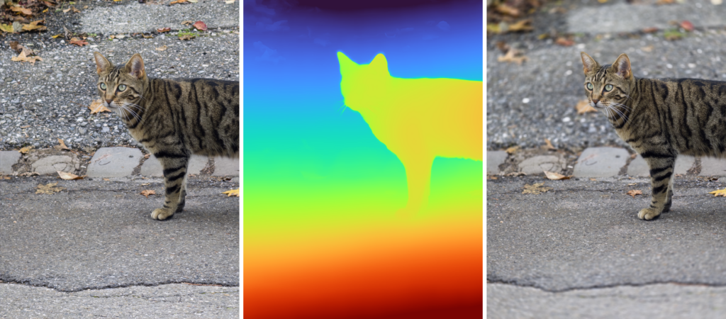
To get high-resolution depth maps, GrainWorks and M-Kamera use MoGe2, a recent research model from Microsoft. It can estimate absolute depth provided the field of view is known (which we can get from EXIF), although it’s not always 100% accurate at a mobile-friendly size. That’s why M-Kamera uses LiDAR data coupled with another, lighter model on top to calibrate MoGe’s output. GrainWorks has to work with any picture, so absolute depth calibration is not possible, and the aperture numbers in GrainWorks are only an approximate indication of what you’d get for a given scene with a 50mm-equivalent lens. On Macs it works slightly better, because a larger and smarter version of the model can be used there.

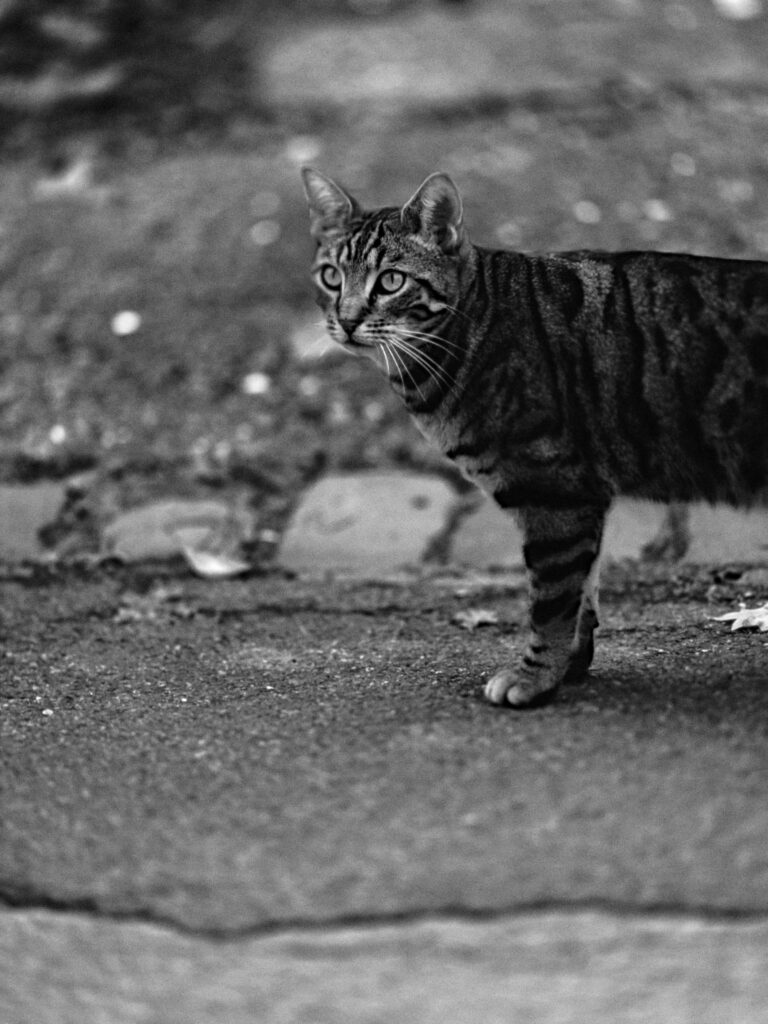
Here is what it makes of a street cat who can’t complain about her picture being posted online (colour encodes distance: warm is near and cool is far):

I mentioned already that getting a larger model to run on a phone is not really feasible. Heard about the RAM crisis? That’s because AI needs a lot of memory, and phones don’t have “a lot” of it.

The workaround is the same as photographing a large map in sections (or Brenizer bokehramas): process the image in tiles. The model first looks at the whole frame to get the overall geometry right, then at overlapping crops at full resolution to get the detail, and the two are combined into one map, which is finally aligned with the edges of the photo. Here is what that does for the whiskers (compared to the original depth resolution):

This allows depth to be recovered more accurately even with the same model, and removes a lot of artefacts in real pictures. Both M-Kamera and GrainWorks use this trick, but M-Kamera has more time to do it (in the background), so you’ve probably never noticed it, whereas in GrainWorks a “Preview quality” label shows up while the tiled depth is being computed and blended.

Rendering the blur

To make it short – both M-Kamera and GrainWorks render honest 3D bokeh. The blur is worked out for every pixel from its own depth using a highly optimized scatter-and-gather renderer. The foreground and the background are blurred separately, and then the depth map is used to guide blending so that the background doesn’t smear around the edges of the subject, while foreground objects can still get unsharp, semi-transparent, see-through edges. Mechanical barrel vignetting (cat’s eyes and swirrrl!) and aperture blades are also simulated. M-Kamera uses variable aperture-dependent vignetting calibrated to a real lens, and the aperture blades disappear wide open, whereas GrainWorks is a bit more aggressive here and uses 5 bladed aperture and a healthy dose of swirly bokeh for a more filmic look. Some other hacks, like highlight boosting, are included to make the bokeh even more realistic.

Colour

Most film simulation apps rely on so-called look-up tables to simulate film colour. Basically, you make a 3D table containing original and target RGB values, and interpolate between the two. The table can, for instance, be obtained by shooting the same scene with an iPhone and a film camera and directly comparing the results. The problem with this approach is that a) the input files must then come from the same camera as used for calibration, and b) the calibration can actually change! Film has a colour response that changes with the actual exposure (and thus light and scene!). Also, GrainWorks was supposed to work with any images, not only those shot on an iPhone.

To overcome these issues, GrainWorks and M-Kamera use a small neural network that looks at a thumbnail of your photo and works out a custom colour table for this picture, which is then applied to the full-resolution version. This model is scene/geometry aware, i.e. it knows when a person or sky is in frame and what the histogram of the given image looks like. It was trained on a mix of paired digital/film images shot by me and some public-domain film scans with no digital counterparts (as an additional unpaired loss term to prevent overfitting on my small dataset). Each stock has its own network, and the filter response is also learned rather than done in a channel mixer.

Grain

The grain is based on the paper by Alasdair Newson et al., which I also use in M-Kamera. The core of the algorithm mimics the random scatter of developed grains in the emulsion, and how the enlarger and your eye average over them. Basically, you scatter grains as random discs of slightly different sizes, place sample points around each pixel, and count how many of them are covered by a grain to compute the pixel intensity. Parameters like the number of discs, size of discs etc. define a model, so in principle both coarse- and fine-grained films can be simulated by simply adjusting the model parameters.

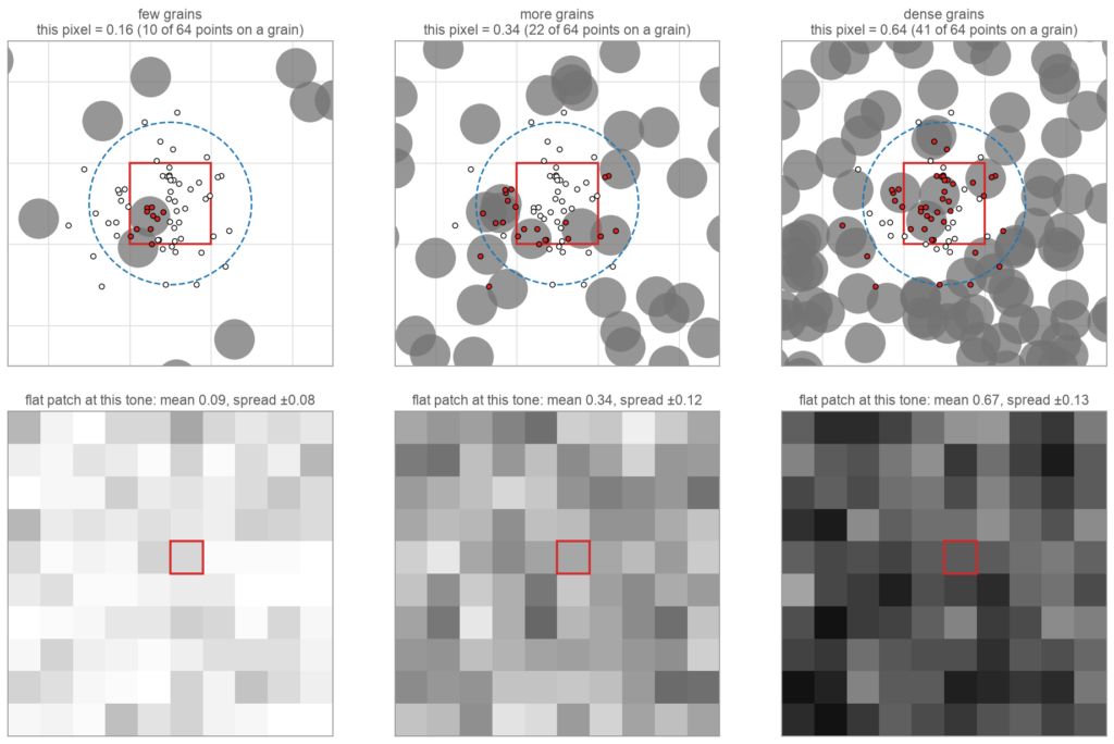
Sounds simple, but there’s a performance catch. The original algorithm is a research tool and takes about half an hour to render a full-size picture even on a workstation, so it had to be simplified and rewritten from scratch to run on a phone’s GPU. The grain of each stock was then tuned automatically to match flat patches of real film scans by varying the model parameters and computing several similarity metrics, followed by a final visual inspection on real film images where part of a flat area was first blurred to the max and then filled with simulated grain.

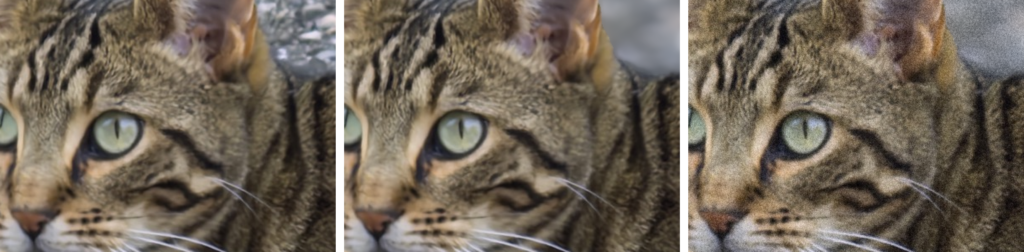
On a real picture it looks like this:

Halation

The recipe is simple: blur the bright parts of each colour channel separately – red the widest and strongest, green much less, blue not at all – and add the glow back onto the picture. Portra gets a lot of it, Tri-X some (as a mono glow), and E100 much less. This time it was tuned visually to match what actual film shows (although it’s tricky to get halation to show up, so the number of images used for tuning is low).

Closing remarks

None of this is “AI making a picture”. AI does only two jobs, guessing the distances and predicting a colour table; everything else is optics and photochemistry simulated as faithfully as I could, which is the astrophysicist in me talking (again). I’m personally quite happy with the results and believe they’re among the best you can get, at least for the film simulation part, even if film simulation can never be perfect. If anyone wants to compare them directly with other simulation apps or film, you’re more than welcome to do so and share your results 🙂

You can find both M-Kamera and GrainWorks: Film Sim & Bokeh on the App Store, and more info at mkamera.app. Feedback of any kind is hugely appreciated, especially failure cases: if you find a picture where the blur goes wrong (and you will, the depth model is good but not perfect!), please send it to su*****@*****ra.app, as that’s how it gets better. Good light!

Here’s a short video of UI in action on the mac:

App in action on a Mac

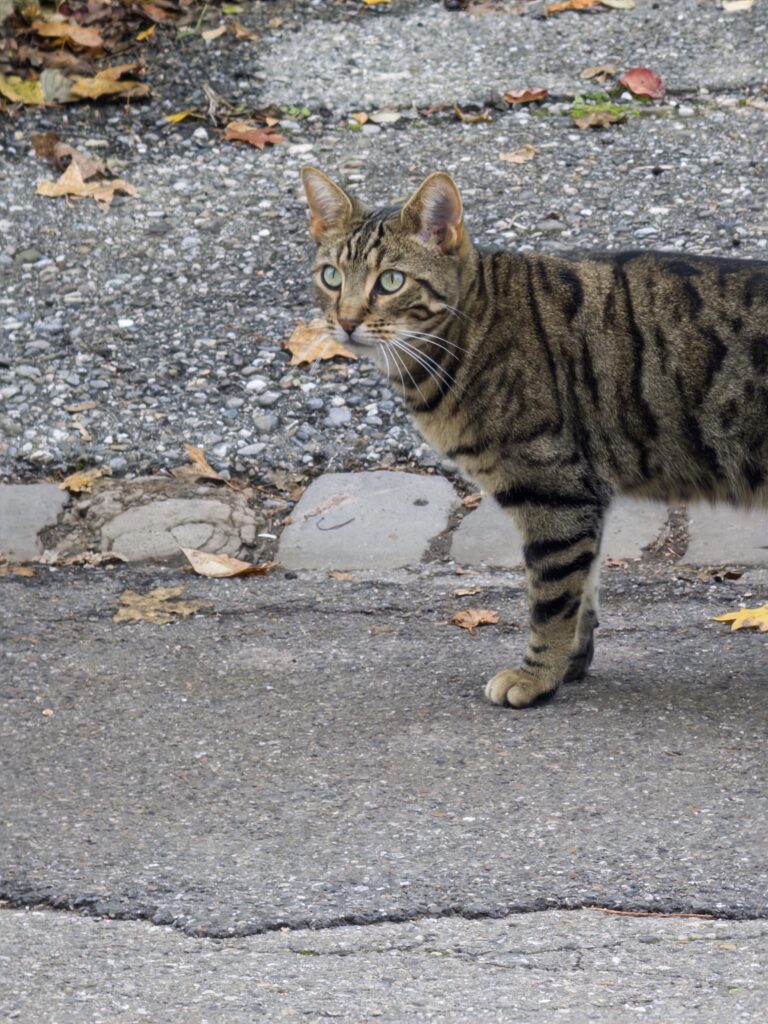
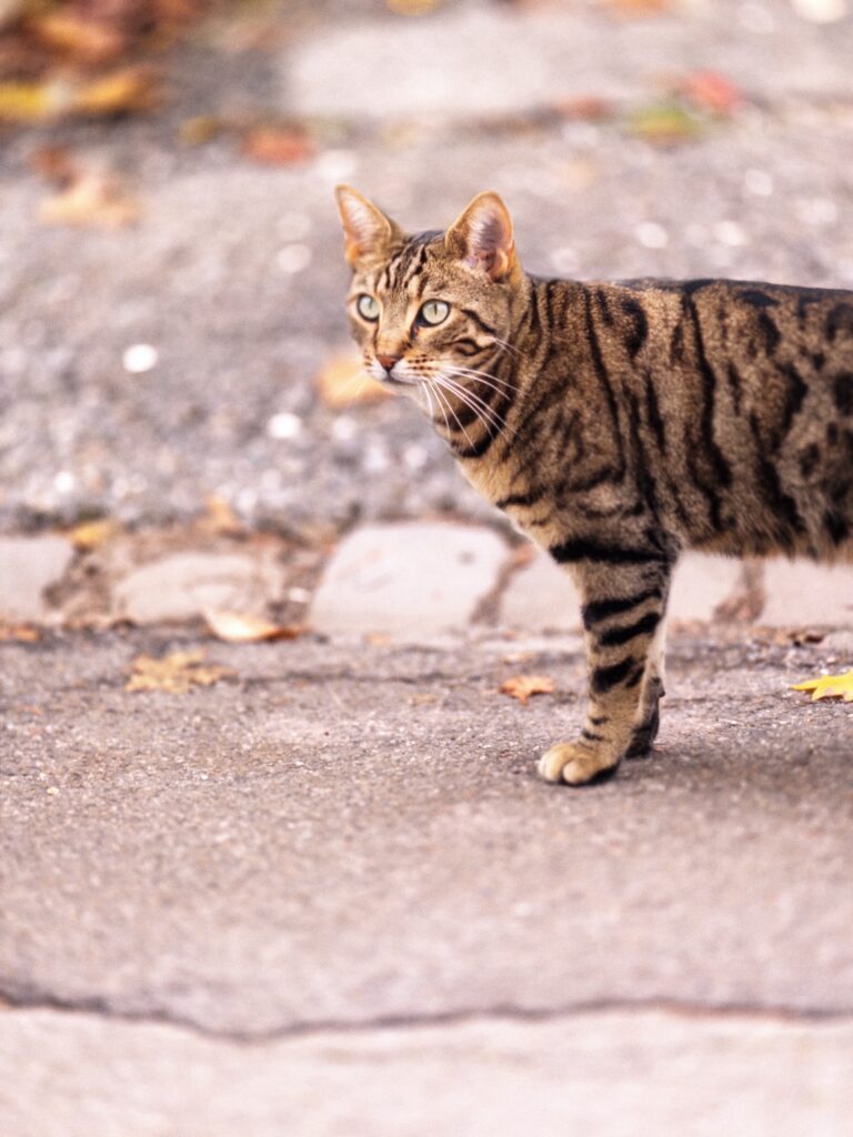
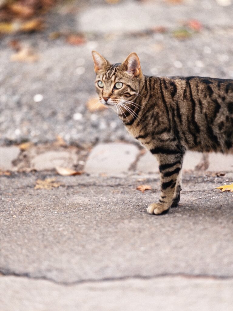
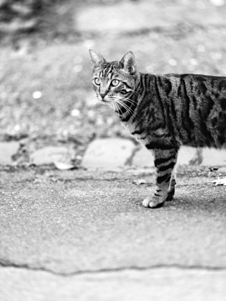
And of course, same cat with all simulations for comparison:

Share this post: