Why Does Colour Negative Film Have an Orange Mask?

I have recently been experimenting with Kodak Aerocolor IV 2460 – a rather unique colour film stock.

Kodak Aerocolor IV (not to be confused with the even more exotic Aerochrome – a discontinued and now eye-wateringly expensive false-color infrared film) is a colour negative film which does not have the usual orange mask. Instead, it has an almost clear base, with a light pink or magenta tint. Kodak’s datasheet (PDF) explains that the film is for “general use in medium- to high-altitude aerial-mapping and aerial-reconnaissance photography,” and because it “does not have integral color masking, direct interpretation can be made from the negative.”

This got me wondering why colour negative film has the orange mask in the first place. I knew the standard explanation, which many of you probably know too: the orange mask compensates for imperfections in the film. But what exactly are these imperfections, and how does the mask compensate? If a film lacks this mask, like Aerocolor, how will that affect its colour rendition? Does the lack of a mask make the film easier to scan? And if colour film is just going to be scanned and not printed in a traditional analogue darkroom, do we even need the mask at all?

I eventually plan to write a proper review of Aerocolor IV, but this article is about why the orange mask exists and what it does. Rather surprisingly, I couldn’t find an online explanation pitched at the level that I wanted. Some are too shallow, while others, which are listed under the “References” section below, are deep, but not so easy for a beginner to understand. So I wrote this article as an in-depth but beginner-friendly explanation and simulation of the orange mask phenomenon.

This article has some simplifying assumptions. For example, some of the relationships (e.g. between exposure and density) are assumed to be linear which is not always the case, and RGB values do not exactly represent human vision or photochemical response. But the basic ideas are still valid, and the model, though simplified, can help us understand how colour negative film records and reproduces colours.

Deconstructing Colour Negative Film

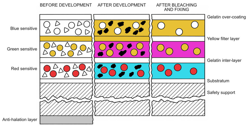
Colour negative film has a number of layers, but for now, we are interested in the three main image-forming layers:

• Blue-sensitive layer (yellow dye)
• Green-sensitive layer (magenta dye)
• Red-sensitive layer (cyan dye).

When the film is exposed to light, developed and fixed, these layers form yellow, magenta and cyan dyes respectively – the complementary colours of the light they record. Generally speaking, the more light a layer is exposed to, the more dye it forms.

Blue-sensitive Layer

Now imagine you have a colour negative film with perfect dyes. (In reality, no dye is perfect, which is why we need the orange mask. But stay with me for now.) And imagine also that you are using this film to photograph this gradient, which goes from black to blue.

Since the film is exposed to blue light only, the Green- and Red-sensitive layers on the film record nothing at all, so no dye is formed in those layers. After development and fixing, the Green- and Red-sensitive layers remain colourless, transparent.

In the Blue-sensitive (yellow dye) layer of the negative, the left edge – black in the original image – is also unexposed and remains transparent. But moving from left to right, the exposure – and therefore the density of yellow dye – increases all the way to the right edge, as shown below.

Incidentally, if we were to invert the colours in Fig 3, we would be right back where we started: the black–blue gradient of Fig 2.

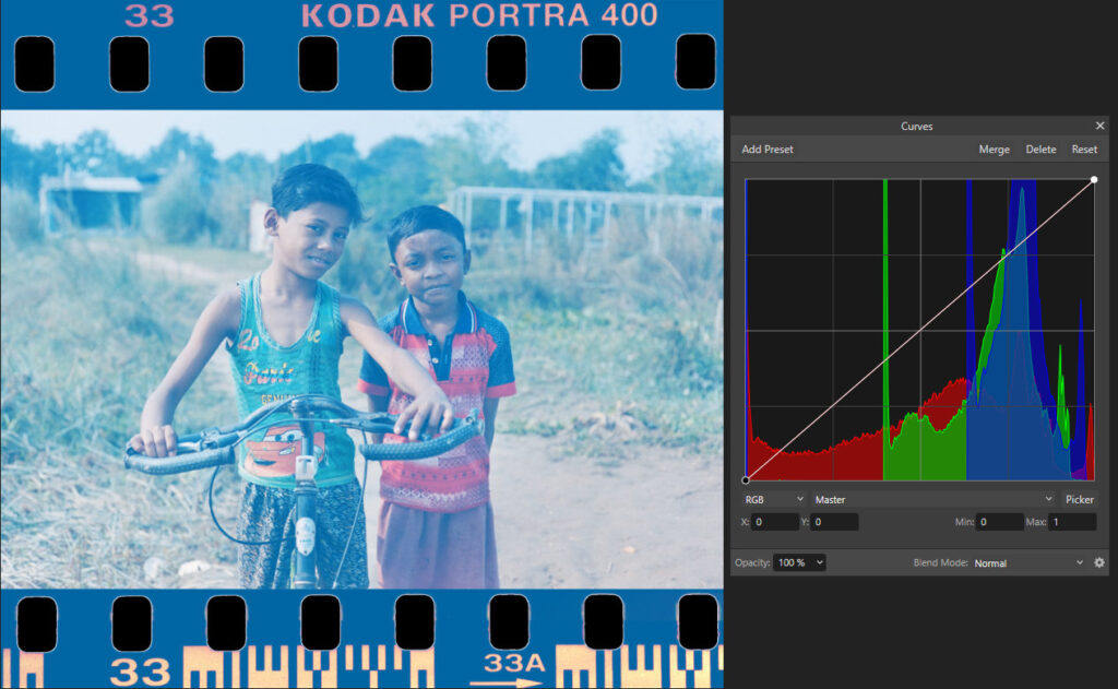
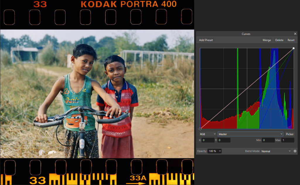
I chose the gradient image because it clearly illustrates how different levels of exposure translate to density in the negative. But some of us find it easier to grasp real-life examples, so here’s a real negative (scanned and inverted), and a simulation of its Blue-sensitive (yellow dye) layer:

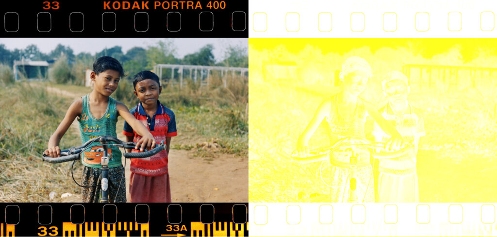
To be clear, the negative is real, but the yellow dye layer is a simulation (the “Technical notes” section below explains how I made these simulations). It’s physically impossible to separate the dye layers in an actual negative, but the simulation is close enough to give us a pretty good idea of what’s happening under the hood.

Note how the dark parts, like the boys’ hair, are nearly transparent in the negative, while the bright parts, like the sky, are a vivid yellow.

Green-sensitive Layer

Now imagine you photograph this gradient which goes from black to green:

This time, the film’s Blue- and Red-sensitive layers will remain unexposed and transparent, but the Green-sensitive (magenta dye) layer will go from transparent to magenta:

So far, as I said, we assumed that the dyes are perfect. And the yellow dye (Blue-sensitive) is indeed close to perfect. But the magenta dye (Green-sensitive) is not.

If you photographed the black–green gradient from Fig 4 using the imperfect dye, the Green-sensitive layer would look something like this (I added a strip at the bottom, to compare with the perfect magenta dye from Fig 5).

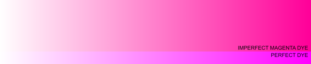
Imagine you hold a piece of magenta-dyed film up against the light. A perfect magenta dye would block green light completely – green being the complement of magenta – and transmit 100% of red and blue light. (In fact, that’s what gives the dye its colour, since red and blue, mixed additively, produce magenta.)

Our imperfect magenta dye transmits red light effectively (which is good), but it blocks a bit of blue (not so good). Blocking blue light has the same visual effect as adding yellow (its complement), so we can also think of the impure dye as magenta with a yellow tint.

If you invert the colours in this image, the left edge will be pure black, just like Fig 4. But the right edge will be a slightly blue-tinted green (0,255,51) as opposed to the pure green (0,255,0) of Fig 4. The colour-rendition has been “polluted” by the imperfection in the magenta dye.

So what’s the big deal – can’t we just subtract the unwanted yellow and get back our pure magenta?

Unfortunately that’s not so easy, because the unwanted blue blockage (yellow tint) is in proportion to the amount of magenta dye. Note how, in Fig 6, the left edge is completely clear (no magenta dye, and no unwanted tint). But as the magenta density increases, the unwanted tint increases too.

The solution is to incorporate a yellow dye coupler into the magenta-forming layer. During development, the coupler loses its yellow colour in proportion to the amount of magenta dye which is formed. Where less magenta dye forms, more of the yellow coupler remains. The result is that the unwanted blue blockage stays approximately constant across the layer, rather than increasing with magenta density. For the purposes of our simplified model, we can think of this as adding a yellow mask which decreases in proportion to the amount of magenta dye that is formed.

So if you photographed the green gradient from Fig 4, the yellow mask, on its own, would look like this:

At the left edge – where the Green-sensitive layer is unexposed and there is no magenta dye – the film base is yellow. As the magenta dye intensifies, the yellow mask clears, becoming transparent at the right edge.

The combination of the imperfect magenta dye and yellow mask would look like this:

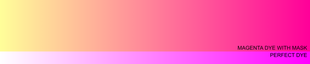
The addition of the mask ensures that the yellow tint is no longer variable, but constant. If you sample the RGB values anywhere on the top strip – e.g. at the left edge (255,255,153), middle (255,127,153) or right edge (255,0,153), you’ll see that the value of the green channel decreases (i.e. magenta increases), but the value of the blue channel (the complement of yellow) remains constant across the gradient.

So in theory, we can subtract a certain amount of yellow from the whole image, and get back a pure magenta tone. Or when inverting the negative, whether as a darkroom print or a scan, we can subtract a certain amount of blue – the complement of yellow.

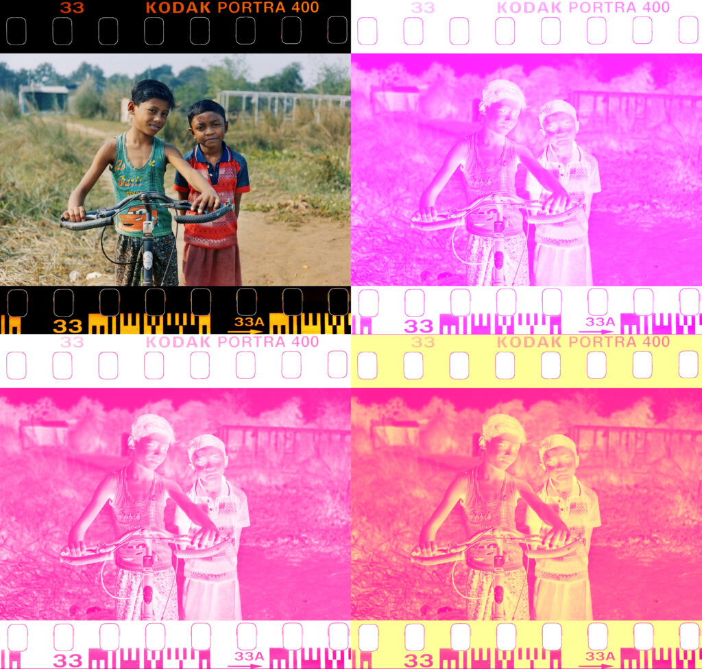
Going back to our real-life negative, here is what the Green-sensitive (magenta dye) layer would look like:

Red-sensitive Layer

Now for the final layer. Let’s say you photograph this gradient which goes from black to red.

The Red-sensitive layer has a cyan dye, which is also imperfect. With a perfect cyan dye, the Red-sensitive layer would have gone from transparent to pure cyan.

A perfect cyan dye would block red light, and transmit 100% of green and blue light. In practice, the cyan dye blocks not just red light, but also a bit of both green and blue. Green and blue combine to form cyan, so what the dye imperfection is doing is to essentially subtract a bit of cyan from the mix, producing a less saturated shade than the ideal case.

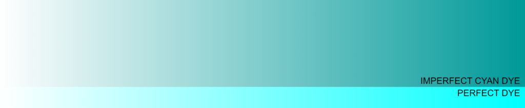
The dye imperfection – subtracting a bit of cyan – is equivalent to adding a light red (red being the complement of cyan).

Like with the magenta-dye imperfection in the Green layer, the fix is to incorporate a light red dye coupler into the cyan-forming layer. During development, the coupler loses its reddish colour in proportion to the amount of cyan dye which is formed. Where less cyan dye forms, more of the reddish coupler remains. The result is that the unwanted blockage stays approximately constant across the layer, rather than increasing with cyan density. For the purposes of our simplified model, we can think of this as adding a light red mask which decreases in proportion to the amount of cyan dye that is formed.

If you now photograph the black–red gradient from Fig 9, here’s what the isolated light-red mask would look like after exposure and development:

In old Kodak literature, this mask is referred to as salmon, which always makes me think of this meme.

The combination of the imperfect cyan dye and reddish mask would look like this:

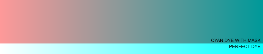
As before, the addition of the mask ensures that the dye-imperfection (reddish tint in this case) is no longer variable, but constant. When the negative is inverted in the darkroom or digitally, the constant reddish tint can be compensated for more easily than the variable tint.

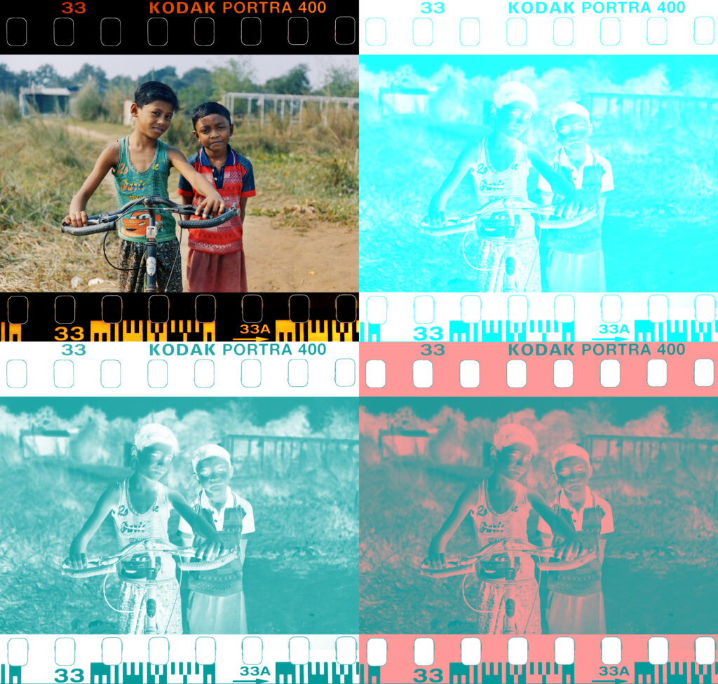
Here’s what the Red-sensitive (cyan dye) layer of our sample negative would look like:

The Combination Mask

So far we looked at coloured gradients. But if we photographed a black–white gradient, the dye layers would in fact look very similar. White light is a combination of blue, green and red, so the Blue-, Green- and Red-sensitive layers would all respond to it in similar ways: clear at the left edge, and maximum density – of yellow, magenta and cyan dye respectively – at the right edge.

If we had perfect dyes, the three layers, thanks to the subtractive colour-mixing property of dyes, would combine to form a gradient ranging from white, through neutral grey, to black – a perfect negative image of the original gradient.

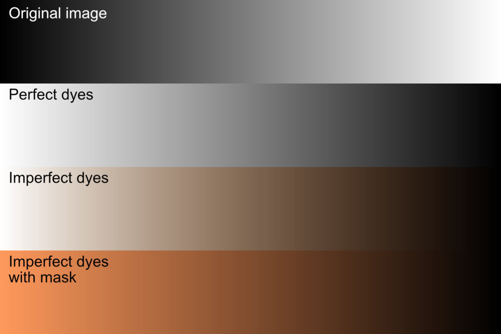
With imperfect dyes, we would get a sepia-tinted gradient. The unwanted yellow tint in the Green-sensitive (magenta dye) layer and the unwanted reddish tint in the Red-sensitive (cyan dye) layer both increase in proportion to exposure, producing sepia.

And with imperfect dyes plus masks, we would get an orange-black gradient – the effect is like looking at a neutral white-black gradient through an orange filter. When inverting the negative image to a positive – either in a darkroom or digitally after scanning – we essentially subtract that orange filter (or add a complementary cyan filter to neutralize it), thus getting back the true colours.

Now let’s look at the three layers of the sample negative, and how they combine to form an image.

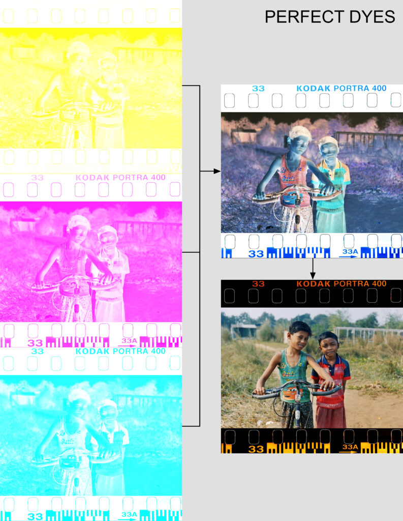
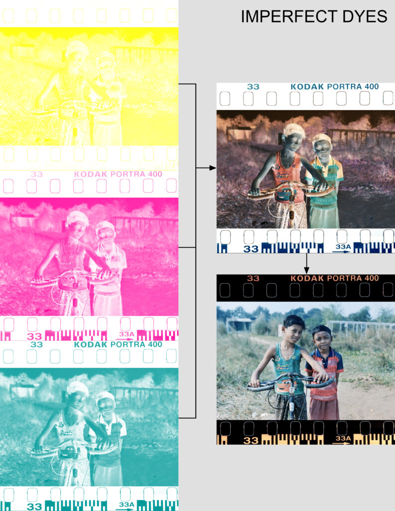
The first comparison (above) is between the hypothetical perfect dyes, and the imperfect dyes. Note that the Blue-sensitive layer (top left) is identical, since the yellow dye is already near-perfect. But the magenta and cyan dye layers have a noticeable tint.

At top right, you can see what the negative would look like if you were to superimpose the three layers and hold them up against the light (for the simulation, I layered them in Affinity using the Multiply blend mode, which has the same effect).

Bottom right is a direct inversion. The ideal dyes produce rich, true colours, while the imperfect dyes create a somewhat faded image. In particular, the greens and reds look less saturated because the corresponding magenta and cyan dyes have more imperfections.

The next comparison (below) is between the hypothetical perfect dyes, and the imperfect dyes with mask.

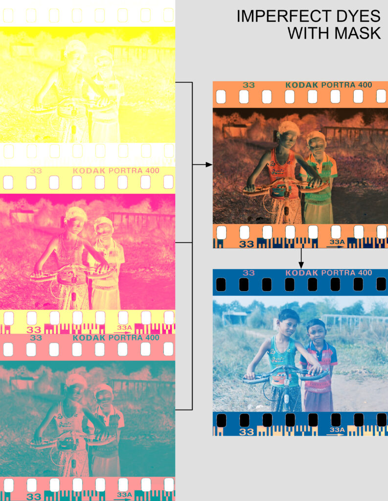
As before, the Blue-sensitive layer (top left) is identical. The yellow and light red masks combine to form the familiar brick-orange film base of a colour negative (top right). When that image is inverted, the result, at first glance, is even further from what we got with imperfect dyes without mask. But this time, we can subtract out a constant amount of cyan, and get back the true colours.

To sum up, the yellow dye in the Blue-sensitive layer is near perfect, but a yellow mask is added to the magenta dye in the Green-sensitive layer, and a light red mask to the cyan dye in the Red-sensitive layer.

Without the mask, the anomalous tint would have been variable – increasing in proportion to dye density, and therefore difficult to eliminate. With the mask, regardless of the level of exposure, we have a consistent tint which is (relatively) easy to subtract out, and thus regain the true colours that we set out to record.

As an analogy, consider how it’s easier to correct for a weighing scale which always shows 10kg more than the true weight, compared to one which shows 5% more than the true weight. In the first case, you simply subtract a known amount. In the second case, you have to do more math. (Compared to my simplistic weighing-scale example, the actual math for colour negatives is even more complicated.)

So if we only scan our negatives, and never print them in the darkroom, does that make the orange mask redundant? Not necessarily. By making the unwanted dye absorption more predictable, the mask makes colour-correction easier, even in a digital workflow. In my follow-up article about Kodak Aerocolor IV, I will explore the pros and cons of scanning and colour-correcting an (almost) clear-base colour negative film.

Technical Notes

I created the gradients with MDiGi tools gradient generator. They are conceptual simulations, not physically accurate renderings of photographic dye layers.

The negative (the photo of the two boys) was made with a Leica M3 and Summicron 50mm f2 lens on Kodak Portra 400 film, scanned with a digital camera with a high-CRI light source as backlight, then inverted and processed in Affinity.

The film-layer simulations were made with a program which I coded in Python. The program can isolate the red, green and blue channels of an image and map them to specified values. For example, for the perfect magenta dye layer, the darkest and lightest values in the green channel were mapped to Hex values FFFFFF (white) and FF00FF (pure magenta) respectively. For the imperfect magenta dye layer with mask, the darkest and lightest values in the green channel were mapped to Hex values FFFF99 and FF0099.

To merge the layers and simulate what the combined negative would look like, I used Affinity’s Multiply blend mode (subtractive colour mixing).

Sources

●  Evans, Hanson & Brewer, Principles of Color Photography (1953)
●  Hunt, The Reproduction of Colour (6th ed, 2004)
●  Collins, The Story of Kodak (1990)
●  Kapecki, ‘Color Photography’ in Peres (ed), Focal Encyclopedia of Photography (4th ed, 2007)
●  Hanson, ‘Color Correction with Colored Couplers’ (1950) 40(3) Journal of the Optical Society of America 166
●  Kodak, Exploring the Color Image (1996)
●  Pritchard, Why Color Negatives Are Orange
●  Dorsky, Why is Color Negative Film Orange?
●  Film Atlas: Eastman Color
●  FilmColors.org: Eastman Color Negative, type 5248
●  FilmColors.org: Eastman Color Negative, type 5250

Share this post: